import numpy as np
import preliz as pz

import gEconpy as ge
import gEconpy.plotting as gp

seed = sum(map(ord, "Intro to gEconpy"))
rng = np.random.default_rng(seed)
Introduction to gEconpy#
gEconpy is a python package for the definition, estimation, and analysis of Dynamic Stochastic General Equlibrium (DSGE) models.
A model begins with a GCN file. This file format was originally introduced by the R package gEcon, written by Karol Podemski and Kaja Retkiewicz-Wijtiwiak. gEconpy has absolutely no affiliation with their project. Note that while GCN files as originally implemented in gEcon are fully compatible with gEconpy, gEconpy also includes many new features that are not backwards compatible.
To show the different features of gEconpy, we will use a simple RBC model. The model is loaded in using the ge.model_from_gcn fucntion.
file_path = "../GCN Files/RBC_backward_compat.gcn"
model = ge.model_from_gcn(file_path, verbose=True)
Model Building Complete.
Found:
	9 equations
	9 variables
		The following variables were eliminated at user request:
			TC_t, U_t
		The following "variables" were defined as constants and have been substituted away:
			mc_t
	1 stochastic shock
		 0 / 1 has a defined prior.
	6 parameters
		 0 / 6 parameters has a defined prior.
	0 parameters to calibrate.
Model appears well defined and ready to proceed to solving.
Model Equations#
All the FoC are saved in the model object and can be manipulated using Sympy if needed
for eq in model.equations:
    display(eq)
Calibrating Relationships#
for eq in model.calibrated_params:
    display(eq)
Model Summary#
To view a summary of the model and the structure of the GCN file that generated it, you can use ge.print_gcn_file. This will let you see the exact blocks defined in the GCN, along with the equations. This is not the final form of the model – first order conditions have not been computed, nor have reductions or simpifications been applied.
ge.print_gcn_file(file_path)
Block: HOUSEHOLD
Definitions
\[u_{t} = - \frac{C_{t}^{1 - \sigma_{C}}}{\sigma_{C} - 1} - \frac{L_{t}^{\sigma_{L} + 1}}{\sigma_{L} + 1}\]
Controls
\[\operatorname{Set}\left(\left[ C_{t}, \ L_{t}, \ I_{t}, \ K_{t}\right]\right)\]
Objective
\[U_{t} = \beta U_{t+1} + u_{t}\]
Constraints
\[C_{t} + I_{t} = K_{t-1} r_{t} + L_{t} w_{t}\]
\[K_{t} = I_{t} - K_{t-1} \left(\delta - 1\right)\]
Calibration
\[\beta = 0.99\]
\[\delta = 0.02\]
\[\sigma_{C} = 1.5\]
\[\sigma_{L} = 2.0\]
Block: FIRM
Controls
\[\operatorname{Set}\left(\left[ K_{t-1}, \ L_{t}\right]\right)\]
Objective
\[TC_{t} = - K_{t-1} r_{t} - L_{t} w_{t}\]
Constraints
\[Y_{t} = A_{t} K_{t-1}^{\alpha} L_{t}^{1 - \alpha}\]
Identities
\[mc_{t} = 1\]
Calibration
\[\alpha = 0.35\]
Block: TECHNOLOGY_SHOCKS
Identities
\[\log{\left(A_{t} \right)} = \rho_{A} \log{\left(A_{t-1} \right)} + \epsilon_{A t}\]
Shocks
\[\operatorname{Set}\left(\left[ \epsilon_{A t}\right]\right)\]
Calibration
\[\rho_{A} = 0.95\]
Solve Steady State#
By default, the steady state is found using a combination of Sympy simplifications and scipy optimizers. It can be slow the first time it is run, but it builds a function which can be reused to re-solve the steady-state much more quickly. This is useful when sampling from the prior or posterior.
ss_res = model.steady_state(how="root")
Steady state found
--------------------------------------------------------------------------------
Optimizer message             The solution converged.
Sum of squared residuals      6.694730077435053e-23
Maximum absoluate error       4.7557513482843206e-12
Gradient L2-norm at solution  3.2123231424772236e-10
Max abs gradient at solution  3.1686400031594175e-10
ge.print_steady_state(ss_res)
A_ss               1.000
C_ss               2.358
I_ss               0.715
K_ss              35.732
L_ss               0.820
Y_ss               3.073
lambda_ss          0.276
r_ss               0.030
w_ss               2.436
Steady State Equations#
If you want to work with the steady state equations, use ge.utilities.eq_to_ss. This sends all variables in an equation to the steady state.
for eq in model.equations:
    display(ge.utilities.eq_to_ss(eq).simplify())
To get the variables themselves, you can use x.to_ss(). For example:
ss_vars = [x.to_ss() for x in model.variables]
ss_vars
[A_ss, C_ss, I_ss, K_ss, L_ss, Y_ss, lambda_ss, r_ss, w_ss]
ss_vars[0]
Linearization#
The first step in solving a DSGE model is to linearize the non-linear system. The model.linearize_model takes symbolic derivatives of your model equations with respect to variables at time \(t-1\) (A matrix), \(t\) (B matrix), \(t+1\) (C matrix), and shocks (D matrix), and evaluates the resulting derivatives at the steady state.
A, B, C, D = model.linearize_model(steady_state_kwargs={"how": "root"})
Steady state found
--------------------------------------------------------------------------------
Optimizer message             The solution converged.
Sum of squared residuals      6.694730077435053e-23
Maximum absoluate error       4.7557513482843206e-12
Gradient L2-norm at solution  3.2123231424772236e-10
Max abs gradient at solution  3.1686400031594175e-10
Matrices are returned as numpy arrays
with np.printoptions(linewidth=1000, precision=3, suppress=True):
    print(A)
[[ 0.     0.     0.     1.076  0.     0.     0.     0.     0.   ]
 [ 0.     0.     0.    35.018  0.     0.     0.     0.     0.   ]
 [ 0.     0.     0.     0.     0.     0.     0.     0.     0.   ]
 [ 0.     0.     0.     0.     0.     0.     0.     0.     0.   ]
 [ 0.     0.     0.     0.     0.     0.     0.     0.     0.   ]
 [ 0.     0.     0.     1.076  0.     0.     0.     0.     0.   ]
 [ 0.     0.     0.    -0.02   0.     0.     0.     0.     0.   ]
 [ 0.     0.     0.     0.853  0.     0.     0.     0.     0.   ]
 [ 0.95   0.     0.     0.     0.     0.     0.     0.     0.   ]]
This is pretty ugly though. You can convert a matrix to a pandas dataframe using ge.matrix_to_dataframe. It will try to guess what the labels should be, but in this case the default guess is wrong. We have to tell it that dim1 (the index) are the model equations, not the variables.
ge.matrix_to_dataframe(A, model, dim1="equation", round=3)
| A | C | I | K | L | Y | lambda | r | w | |
|---|---|---|---|---|---|---|---|---|---|
| Equation 0 | 0.00 | 0.0 | 0.0 | 1.076 | 0.0 | 0.0 | 0.0 | 0.0 | 0.0 |
| Equation 1 | 0.00 | 0.0 | 0.0 | 35.018 | 0.0 | 0.0 | 0.0 | 0.0 | 0.0 |
| Equation 2 | 0.00 | 0.0 | 0.0 | 0.000 | 0.0 | 0.0 | 0.0 | 0.0 | 0.0 |
| Equation 3 | 0.00 | 0.0 | 0.0 | 0.000 | 0.0 | 0.0 | 0.0 | 0.0 | 0.0 |
| Equation 4 | 0.00 | 0.0 | 0.0 | 0.000 | 0.0 | 0.0 | 0.0 | 0.0 | 0.0 |
| Equation 5 | 0.00 | 0.0 | 0.0 | 1.076 | 0.0 | 0.0 | 0.0 | 0.0 | 0.0 |
| Equation 6 | 0.00 | 0.0 | 0.0 | -0.020 | 0.0 | 0.0 | 0.0 | 0.0 | 0.0 |
| Equation 7 | 0.00 | 0.0 | 0.0 | 0.853 | 0.0 | 0.0 | 0.0 | 0.0 | 0.0 |
| Equation 8 | 0.95 | 0.0 | 0.0 | 0.000 | 0.0 | 0.0 | 0.0 | 0.0 | 0.0 |
By default, the parameter values set in the GCN file will be used. You are always allowed to set new values, though. For example, we can change \(\rho\) from 0.95 to 0.5:
A, B, C, D = model.linearize_model(rho_A=0.5, steady_state_kwargs={"how": "root"})
Steady state found
--------------------------------------------------------------------------------
Optimizer message             The solution converged.
Sum of squared residuals      6.258140628923231e-32
Maximum absoluate error       2.220446049250313e-16
Gradient L2-norm at solution  1.5915716198724126e-14
Max abs gradient at solution  1.5862311464331924e-14
Notice that the value of \(A\) at Equation 8 is now 0.5
ge.matrix_to_dataframe(A, model, dim1="equation", round=3)
| A | C | I | K | L | Y | lambda | r | w | |
|---|---|---|---|---|---|---|---|---|---|
| Equation 0 | 0.0 | 0.0 | 0.0 | 1.076 | 0.0 | 0.0 | 0.0 | 0.0 | 0.0 |
| Equation 1 | 0.0 | 0.0 | 0.0 | 35.018 | 0.0 | 0.0 | 0.0 | 0.0 | 0.0 |
| Equation 2 | 0.0 | 0.0 | 0.0 | 0.000 | 0.0 | 0.0 | 0.0 | 0.0 | 0.0 |
| Equation 3 | 0.0 | 0.0 | 0.0 | 0.000 | 0.0 | 0.0 | 0.0 | 0.0 | 0.0 |
| Equation 4 | 0.0 | 0.0 | 0.0 | 0.000 | 0.0 | 0.0 | 0.0 | 0.0 | 0.0 |
| Equation 5 | 0.0 | 0.0 | 0.0 | 1.076 | 0.0 | 0.0 | 0.0 | 0.0 | 0.0 |
| Equation 6 | 0.0 | 0.0 | 0.0 | -0.020 | 0.0 | 0.0 | 0.0 | 0.0 | 0.0 |
| Equation 7 | 0.0 | 0.0 | 0.0 | 0.853 | 0.0 | 0.0 | 0.0 | 0.0 | 0.0 |
| Equation 8 | 0.5 | 0.0 | 0.0 | 0.000 | 0.0 | 0.0 | 0.0 | 0.0 | 0.0 |
Computing the steady state might be expensive if your model is much larger. If you’ve already computed the steady state, you can give it to linearize_model. This skip re-solving the steady state.
Warning
Be careful providing a steady state!
If you pass new parameter values together with a pre-computed steady state, you must ensure that they agree! If you compute the steady state using one set of parameters, then linearize with another set of parameters, the solution will not be correct. No checking is done to ensure consistency!
A, B, C, D = model.linearize_model(steady_state=ss_res)
Here’s an example of an inconsistent steady state and linearization. If I change \(\beta\) from the default (0.99) to a new value value, gEconpy will:
Compute symbolic derivatives of the system of equations (no values are involved at this point)
Cast all variables to the steady state
Plug in the steady state values you provided! This will be consistent with \(\beta = 0.99\)
Plug in the parameter values you requested. This will be consistent with \(\beta = 0.9\)
As you can see, no errors or warnings are raised, but this linearized matrix is wrong!
A_wrong, B_wrong, C_wrong, D_wrong = model.linearize_model(steady_state=ss_res, beta=0.9)
Here are is the difference between the right and wrong matrices. Since we messed up \(\beta\), the relevant matrix is C – derivatives with respect to the variables at time \(t+1\).
ge.matrix_to_dataframe(C - C_wrong, model, dim1="equation").style.format(precision=3).background_gradient(cmap="YlGn")
| A | C | I | K | L | Y | lambda | r | w | |
|---|---|---|---|---|---|---|---|---|---|
| Equation 0 | 0.000 | 0.000 | 0.000 | 0.000 | 0.000 | 0.000 | 0.000 | 0.000 | 0.000 |
| Equation 1 | 0.000 | 0.000 | 0.000 | 0.000 | 0.000 | 0.000 | 0.000 | 0.000 | 0.000 |
| Equation 2 | 0.000 | 0.000 | 0.000 | 0.000 | 0.000 | 0.000 | 0.000 | 0.000 | 0.000 |
| Equation 3 | 0.000 | 0.000 | 0.000 | 0.000 | 0.000 | 0.000 | 0.000 | 0.000 | 0.000 |
| Equation 4 | 0.000 | 0.000 | 0.000 | 0.000 | 0.000 | 0.000 | 0.025 | 0.001 | 0.000 |
| Equation 5 | 0.000 | 0.000 | 0.000 | 0.000 | 0.000 | 0.000 | 0.000 | 0.000 | 0.000 |
| Equation 6 | 0.000 | 0.000 | 0.000 | 0.000 | 0.000 | 0.000 | 0.000 | 0.000 | 0.000 |
| Equation 7 | 0.000 | 0.000 | 0.000 | 0.000 | 0.000 | 0.000 | 0.000 | 0.000 | 0.000 |
| Equation 8 | 0.000 | 0.000 | 0.000 | 0.000 | 0.000 | 0.000 | 0.000 | 0.000 | 0.000 |
Perturbation Solution#
Like the steady state solution, the perturbation solution constructs a function to solve linearized system via perturbation.
Following Dynare, the default pertubation solver is Cycle Reduction, implemented in Numba for faster execution. You can also ask for Gensys if you wish. The original gEcon used Gensys.
Like linearize_model, you can provide a steady state result to solve_model. You can also ask for parameter updates by passing parameter names as keyword arguments. The same warnings about consistency between the provided steady state and parameter updates apply here!
T, R = model.solve_model(steady_state=ss_res)
Solution found, sum of squared residuals: 0.000000000
Norm of deterministic part: 0.000000000
Norm of stochastic part: 0.000000000
Also like linearize_model, if you don’t pass steady_state, it will automatically re-compute it.
T_gensys, R_gensys = model.solve_model(solver="gensys", steady_state_kwargs={"how": "root"})
Steady state found
--------------------------------------------------------------------------------
Optimizer message             The solution converged.
Sum of squared residuals      6.694730077435053e-23
Maximum absoluate error       4.7557513482843206e-12
Gradient L2-norm at solution  3.2123231424772236e-10
Max abs gradient at solution  3.1686400031594175e-10
Gensys return codes: 1 1 0, with the following meaning:
Gensys found a unique solution.
Policy matrices have been stored in attributes model.P, model.Q, model.R, and model.S
Norm of deterministic part: 0.000000000
Norm of stochastic part: 0.000000000
Both gensys and cycle_reduction should give the same answer
np.allclose(T, T_gensys), np.allclose(R, R_gensys)
(True, True)
Like linearize_model, solve_model will return numpy arrays. You can change them to a pandas dataframe using ge.matrix_to_dataframe. In this case, the guess about the rows and columns is correct.
Note that only two columns have non-zero entries. This is because \(A\) and \(K\) are the state variables. All of the zeros are associated with jumper variables.
ge.matrix_to_dataframe(T, model).style.format(precision=2).background_gradient(cmap="YlGn")
| A | C | I | K | L | Y | lambda | r | w | |
|---|---|---|---|---|---|---|---|---|---|
| A | 0.95 | -0.00 | -0.00 | 0.00 | -0.00 | -0.00 | -0.00 | -0.00 | -0.00 |
| C | 0.31 | 0.00 | 0.00 | 0.48 | 0.00 | 0.00 | 0.00 | 0.00 | 0.00 |
| I | 3.64 | -0.00 | -0.00 | -0.51 | -0.00 | -0.00 | -0.00 | -0.00 | -0.00 |
| K | 0.07 | -0.00 | -0.00 | 0.97 | -0.00 | -0.00 | -0.00 | -0.00 | -0.00 |
| L | 0.21 | 0.00 | 0.00 | -0.16 | 0.00 | 0.00 | 0.00 | 0.00 | 0.00 |
| Y | 1.08 | 0.00 | 0.00 | 0.25 | 0.00 | 0.00 | 0.00 | 0.00 | 0.00 |
| lambda | -0.46 | 0.00 | 0.00 | -0.72 | 0.00 | 0.00 | 0.00 | 0.00 | 0.00 |
| r | 1.08 | 0.00 | 0.00 | -0.75 | 0.00 | 0.00 | 0.00 | 0.00 | 0.00 |
| w | 0.88 | 0.00 | 0.00 | 0.40 | 0.00 | 0.00 | 0.00 | 0.00 | 0.00 |
The \(R\) matrix maps the shocks to the different states in the economy. In this case, we expect everything is affected by a total factor productivity shock. And since the law of motion of technology is \(\ln A_t = \rho_A \ln A_{t-1} + \epsilon_{A,t}\), it’s a nice sanity check to see the effect of \(\epsilon_A\) on \(A_t\) is 1.
ge.matrix_to_dataframe(R, model).style.format(precision=2).background_gradient(cmap="YlGn")
| epsilon_A | |
|---|---|
| A | 1.00 |
| C | 0.33 |
| I | 3.83 |
| K | 0.08 |
| L | 0.22 |
| Y | 1.14 |
| lambda | -0.49 |
| r | 1.14 |
| w | 0.92 |
Blanchard-Kahn Conditions#
After you have a perturbation solution, you can check the Eigenvalues of the system to make sure the BK conditions are satisfied.
The output shows the eigenvalues computed by gensys: the modulus, real part, and imaginary part.
ge.check_bk_condition(model, steady_state=ss_res);
Model solution has 2 eigenvalues greater than one in modulus and 2 forward-looking variables.
Blanchard-Kahn condition is satisfied.
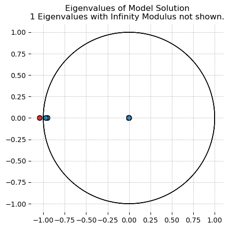
You can also visualize the Eigenvalues using plot_eigenvalues in the plotting functions.
gp.plot_eigenvalues(model, linearize_model_kwargs={"steady_state": ss_res});
Model solution has 2 eigenvalues greater than one in modulus and 2 forward-looking variables.
Blanchard-Kahn condition is satisfied.
Model Statistics#
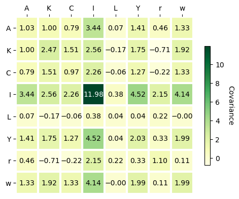
Functions to compute the stationary covariance matrix, as well as autocovariances for each variable, are also available.
cov = np.eye(1) * 0.1
sigma = ge.stationary_covariance_matrix(model, T=T, R=R, shock_cov_matrix=cov)
acorr = ge.autocovariance_matrix(model, T=T, R=R, shock_cov_matrix=np.eye(1), n_lags=30)
sigma.style.format(precision=2).background_gradient(cmap="YlGn")
| A | C | I | K | L | Y | lambda | r | w | |
|---|---|---|---|---|---|---|---|---|---|
| A | 1.03 | 0.79 | 3.44 | 1.00 | 0.07 | 1.41 | -1.18 | 0.46 | 1.33 |
| C | 0.79 | 0.97 | 2.26 | 1.51 | -0.06 | 1.27 | -1.46 | -0.22 | 1.33 |
| I | 3.44 | 2.26 | 11.98 | 2.56 | 0.38 | 4.52 | -3.39 | 2.15 | 4.14 |
| K | 1.00 | 1.51 | 2.56 | 2.47 | -0.17 | 1.75 | -2.26 | -0.71 | 1.92 |
| L | 0.07 | -0.06 | 0.38 | -0.17 | 0.04 | 0.04 | 0.09 | 0.22 | -0.00 |
| Y | 1.41 | 1.27 | 4.52 | 1.75 | 0.04 | 2.03 | -1.90 | 0.33 | 1.99 |
| lambda | -1.18 | -1.46 | -3.39 | -2.26 | 0.09 | -1.90 | 2.18 | 0.33 | -2.00 |
| r | 0.46 | -0.22 | 2.15 | -0.71 | 0.22 | 0.33 | 0.33 | 1.10 | 0.11 |
| w | 1.33 | 1.33 | 4.14 | 1.92 | -0.00 | 1.99 | -2.00 | 0.11 | 1.99 |
Unlike the stationary covariance, the computed autocovariances will be returned as an xarray with a lag dimension. This lets you inspect correlations between all combinations of variables and timesteps.
You can also plot the covaraince matrix as a heatmap using gp.plot_covariance_heatmap. This is basically the same as the styled pandas dataframe, but you can pick which one you think is prettier!
gp.plot_covariance_matrix(
    sigma,
    ["A", "K", "C", "I", "L", "Y", "r", "w"],
    figsize=(5, 5),
    cbar_kw={"shrink": 0.5},
);
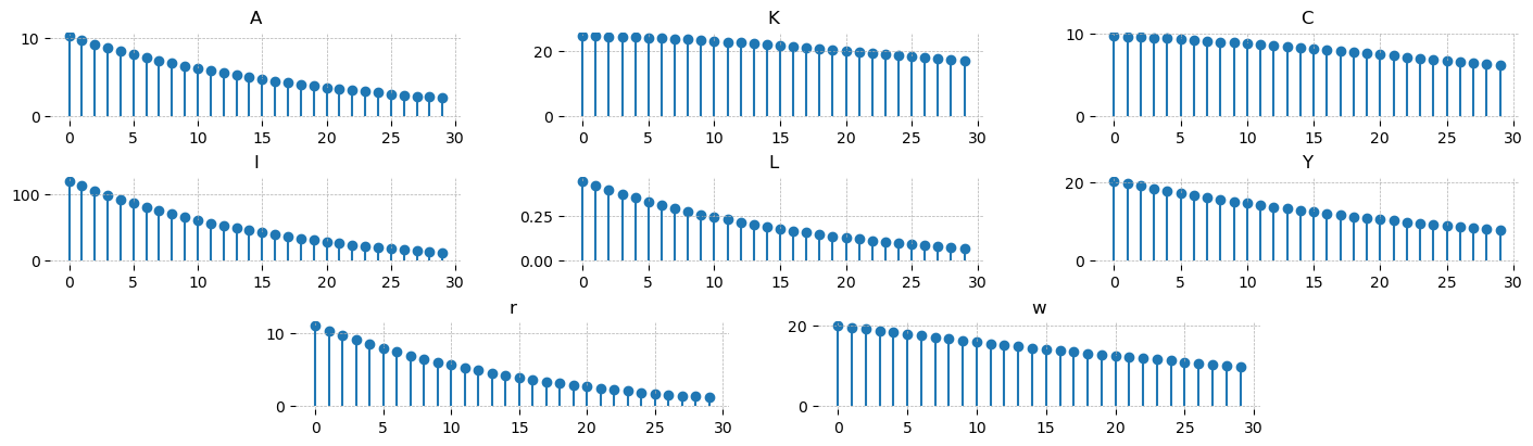
Similarly, there is a function to plot the autocorrelation functions, plot_acf. This only plots self-autocorrelations. For the off-diagonals, you will need to hand-roll something.
gp.plot_acf(acorr, vars_to_plot=["A", "K", "C", "I", "L", "Y", "r", "w"], n_cols=3);
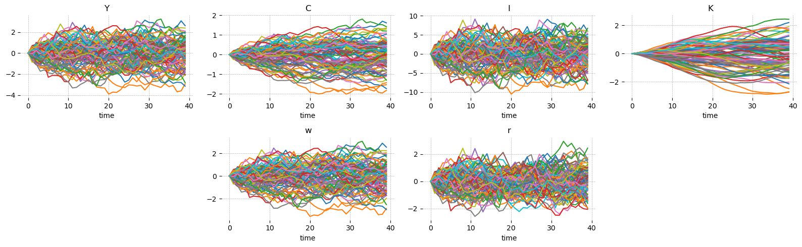
Simulation#
You can simulate the model by passing a covariance matrix for the shocks. The default is a spaghetti plot, but you can also ask for confidence intervals if you prefer a cleaner look.
simulation = ge.simulate(model, T, R, shock_cov_matrix=cov, n_simulations=100, random_seed=rng)
gp.plot_simulation(simulation, vars_to_plot=["Y", "C", "I", "K", "w", "r"], n_cols=4, figsize=(16, 5));
The confidence intervals need plenty of simulations or else they come out looking quite “jagged”.
simulation = ge.simulate(
    model,
    T,
    R,
    shock_cov_matrix=cov,
    n_simulations=100_000,
    simulation_length=100,
    random_seed=rng,
)

gp.plot_simulation(
    simulation,
    vars_to_plot=["Y", "C", "I", "K", "w", "r"],
    ci=0.95,
    n_cols=4,
    figsize=(16, 5),
);
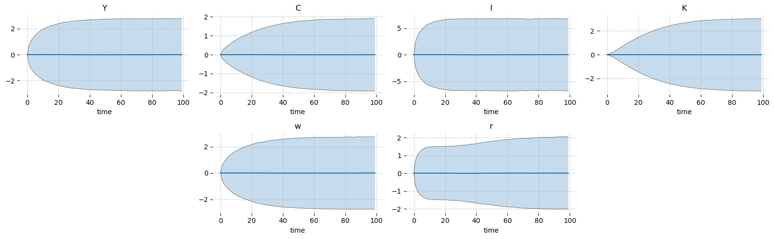
With a large number of simulations you can also compute sample statistics and verify the stationary solution. Evidently they match to about the 2nd decimal place with 10_000 samples at T=99. One could extend simulation_length and increase n_simulations to obtain more accurate estimates.
import pandas as pd

tols = [1e-1, 1e-2, 1e-3, 1e-4, 1e-5]
accuracy_df = pd.DataFrame(0, columns=tols, index=[x.base_name for x in model.variables])
for tol in tols:
    accuracy_df[tol] = ((np.cov(simulation.isel(time=-1).values.T) - sigma).abs() < tol).all()
print("Absolute difference between stationary covariance matrix and sample covariance matrix is less than:")
print(accuracy_df.to_string())
Absolute difference between stationary covariance matrix and sample covariance matrix is less than:
        0.10000  0.01000  0.00100  0.00010  0.00001
A          True     True    False    False    False
C          True    False    False    False    False
I          True    False    False    False    False
K          True    False    False    False    False
L          True     True    False    False    False
Y          True    False    False    False    False
lambda     True    False    False    False    False
r          True    False    False    False    False
w          True    False    False    False    False
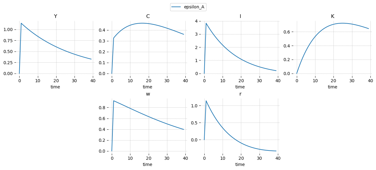
Impulse Response Functions#
They are impulse repsonse functions. Not much to say. The plots start from 0 and the shock enters at 1, which is different from Dynare, which starts the plot at the period the shock enters. The irf object returned by the model.impulse_response_function method is an xarray.Dataset with dimensions (shock, time, variable).
irf = ge.impulse_response_function(model, T=T, R=R, shock_size={"epsilon_A": 1.0})
type(irf)
xarray.core.dataarray.DataArray
irf.dims
('shock', 'time', 'variable')
To plot the IRFs, use gEconpy.plotting.plot_irf. You can request only specific variables using vars_to_plot, and shocks_to_plot to select specific shocks. There’s only one shock in this case, so we don’t use shocks_to_plot.
gp.plot_irf(
    irf,
    vars_to_plot=["Y", "C", "I", "K", "w", "r"],
    n_cols=4,
    figsize=(12, 5),
    legend=True,
);
Covnert to Dynare#
Since Dynare remains the gold standard for DSGE model analysis, gEconpy can convert the model into a Dynare .mod file.
Initial values are set to the steady-state we already computed. Of course you’re free to modify the generated mod file as you like after you copy it over to MatLab.
print(ge.make_mod_file(model))
var A, C, I, K, L, Y, lambda, r, w;

varexo epsilon_A;

parameters alpha, beta, delta, rho_A, sigma_C, sigma_L;

alpha = 0.350;
beta = 0.990;
delta = 0.020;
rho_A = 0.950;
sigma_C = 1.500;
sigma_L = 2.000;


model;

-C - I + K(-1) * r + L * w;
I - K + K(-1) * (1 - delta);
-lambda + C ^ (-sigma_C);
-L ^ sigma_L + lambda * w;
beta * (lambda(+1) * r(+1) - lambda(+1) * (delta - 1)) - lambda;
A * K(-1) ^ alpha * L ^ (1 - alpha) - Y;
alpha * A * K(-1) ^ (alpha - 1) * L ^ (1 - alpha) - r;
A * K(-1) ^ alpha * L ^ (-alpha) * (1 - alpha) - w;
rho_A * log(A(-1)) + epsilon_A - log(A);

end;

initval;
A = 1.000;
C = 2.358;
I = 0.715;
K = 35.732;
L = 0.820;
Y = 3.073;
lambda = 0.276;
r = 0.030;
w = 2.436;

end;

steady;
resid;

check(qz_zero_threshold=1e-20);

shocks;
var epsilon_A;
stderr 0.01;

end;

stoch_simul(order=1, irf=100, qz_zero_threshold=1e-20);
Adding a steady state block#
RBC_backward_compat.gcn shows the “basic” features of gEconpy using a file that is completely backwards compatible with the R package gEcon. There are many more features you can and should take advantage of!
The first one is that you can provide an analytical steady state in your GCN file via a steady_state block. You’re even allow to pass a partial steady state. For an example of that, see the multiple households case study
file_path = "../GCN Files/RBC.gcn"
model = ge.model_from_gcn(file_path, verbose=True)
Model Building Complete.
Found:
	9 equations
	9 variables
		The following variables were eliminated at user request:
			TC_t, U_t
		The following "variables" were defined as constants and have been substituted away:
			mc_t
	1 stochastic shock
		 0 / 1 has a defined prior.
	6 parameters
		 6 / 6 parameters has a defined prior.
	0 parameters to calibrate.
Model appears well defined and ready to proceed to solving.
Steady-State Equations#
In this case, I’ve entered the entire steady state system in the GCN file. If only a partial system is provided, the provided equations will be used to shrink down the number of variables the optimizer needs to look for. gEconpy can use either root finding or loss minimization algorithms to numerically find the steady state, so provided equations don’t need to result in simplification down to a square system!
The most ergonomic way to view the provided equations is to look at the output of print_gcn_file. Notice that there is now a steady_state block. Expand it to see the steady state equations as they were entered in the GCN.
ge.print_gcn_file(file_path)
Block: steady_state
Identities
\[A_{ss} = 1\]
\[mc_{ss} = 1\]
\[r_{ss} = \delta - 1 + \frac{1}{\beta}\]
\[w_{ss} = - \left(\frac{\alpha}{r_{ss}}\right)^{- \frac{\alpha}{\alpha - 1}} \left(\alpha - 1\right)\]
\[Y_{ss} = \left(w_{ss} \left(- \frac{w_{ss}}{\alpha - 1}\right)^{\sigma_{L}}\right)^{\frac{1}{\sigma_{C} + \sigma_{L}}} \left(- \frac{r_{ss}}{\alpha \delta - r_{ss}}\right)^{\frac{\sigma_{C}}{\sigma_{C} + \sigma_{L}}}\]
\[I_{ss} = \frac{\alpha \delta Y_{ss}}{r_{ss}}\]
\[C_{ss} = Y_{ss}^{\frac{\left(-1\right) \sigma_{L}}{\sigma_{C}}} \left(w_{ss}^{\sigma_{L} + 1} \left(1 - \alpha\right)^{- \sigma_{L}}\right)^{\frac{1}{\sigma_{C}}}\]
\[K_{ss} = \frac{\alpha Y_{ss} mc_{ss}}{r_{ss}}\]
\[L_{ss} = - \frac{Y_{ss} mc_{ss} \left(\alpha - 1\right)}{w_{ss}}\]
\[U_{ss} = \frac{\frac{C_{ss}^{1 - \sigma_{C}}}{\sigma_{C} - 1} + \frac{L_{ss}^{\sigma_{L} + 1}}{\sigma_{L} + 1}}{\beta - 1}\]
\[\lambda_{ss} = C_{ss}^{- \sigma_{C}}\]
\[TC_{ss} = - K_{ss} r_{ss} - L_{ss} w_{ss}\]
Block: HOUSEHOLD
Definitions
\[u_{t} = - \frac{C_{t}^{1 - \sigma_{C}}}{\sigma_{C} - 1} - \frac{L_{t}^{\sigma_{L} + 1}}{\sigma_{L} + 1}\]
Controls
\[\operatorname{Set}\left(\left[ C_{t}, \ L_{t}, \ I_{t}, \ K_{t}\right]\right)\]
Objective
\[U_{t} = \beta U_{t+1} + u_{t}\]
Constraints
\[C_{t} + I_{t} = K_{t-1} r_{t} + L_{t} w_{t}\]
\[K_{t} = I_{t} - K_{t-1} \left(\delta - 1\right)\]
Calibration
\[\beta = 0.99\]
\[\delta = 0.02\]
\[\sigma_{C} = 1.5\]
\[\sigma_{L} = 2.0\]
Block: FIRM
Controls
\[\operatorname{Set}\left(\left[ K_{t-1}, \ L_{t}\right]\right)\]
Objective
\[TC_{t} = - K_{t-1} r_{t} - L_{t} w_{t}\]
Constraints
\[Y_{t} = A_{t} K_{t-1}^{\alpha} L_{t}^{1 - \alpha}\]
Identities
\[mc_{t} = 1\]
Calibration
\[\alpha = 0.35\]
Block: TECHNOLOGY_SHOCKS
Identities
\[\log{\left(A_{t} \right)} = \rho_{A} \log{\left(A_{t-1} \right)} + \epsilon_{A t}\]
Shocks
\[\operatorname{Set}\left(\left[ \epsilon_{A t}\right]\right)\]
Calibration
\[\rho_{A} = 0.95\]
Solve Steady State#
Since the entire steady state is provided, There is no need to do any numerical optimization. The values are just computed and returned.
ss_res = model.steady_state()
ge.print_steady_state(ss_res)
A_ss               1.000
C_ss               2.358
I_ss               0.715
K_ss              35.732
L_ss               0.820
Y_ss               3.073
lambda_ss          0.276
r_ss               0.030
w_ss               2.436
It is still possible for the anayltic solution to fail of course – this can happen if you set parameters to bad values (like \(\alpha > 1\) or something). You can always check ss_res.success to make sure everything worked.
ss_res.success
True
Perturbation Solution#
Linearization and perturbation can be done as normal. The steady state function is now very cheap, so I don’t recommend passing the steady state to these functions in this case, but of course you still can. If you don’t, you will not have to worry about the “gotcha” from mismatched parameters.
T, R = model.solve_model()
Solution found, sum of squared residuals: 0.000000000
Norm of deterministic part: 0.000000000
Norm of stochastic part: 0.000000000
==================== T ====================
| A | C | I | K | L | Y | lambda | r | w | |
|---|---|---|---|---|---|---|---|---|---|
| A | 0.950000 | -0.0 | -0.0 | 2.756553e-17 | -0.0 | -0.0 | -0.0 | -0.0 | -0.0 |
| C | 0.309657 | 0.0 | 0.0 | 4.787472e-01 | 0.0 | 0.0 | 0.0 | 0.0 | 0.0 |
| I | 3.640697 | -0.0 | -0.0 | -5.127277e-01 | -0.0 | -0.0 | -0.0 | -0.0 | -0.0 |
| K | 0.072814 | -0.0 | -0.0 | 9.697454e-01 | -0.0 | -0.0 | -0.0 | -0.0 | -0.0 |
| L | 0.206602 | 0.0 | 0.0 | -1.566471e-01 | 0.0 | 0.0 | 0.0 | 0.0 | 0.0 |
| Y | 1.084291 | 0.0 | 0.0 | 2.481794e-01 | 0.0 | 0.0 | 0.0 | 0.0 | 0.0 |
| lambda | -0.464485 | 0.0 | 0.0 | -7.181208e-01 | 0.0 | 0.0 | 0.0 | 0.0 | 0.0 |
| r | 1.084291 | 0.0 | 0.0 | -7.518206e-01 | 0.0 | 0.0 | 0.0 | 0.0 | 0.0 |
| w | 0.877689 | 0.0 | 0.0 | 4.048265e-01 | 0.0 | 0.0 | 0.0 | 0.0 | 0.0 |
==================== R ====================
| epsilon_A | |
|---|---|
| A | 1.000000 |
| C | 0.325955 |
| I | 3.832313 |
| K | 0.076646 |
| L | 0.217476 |
| Y | 1.141359 |
| lambda | -0.488932 |
| r | 1.141359 |
| w | 0.923883 |
BK Conditions#
Nothing changes about checking BK conditions.
gp.plot_eigenvalues(model);
Model solution has 2 eigenvalues greater than one in modulus and 2 forward-looking variables.
Blanchard-Kahn condition is satisfied.
Impulse Response Functions#
Nor in making and plotting IRFs
irf = ge.impulse_response_function(model, T=T, R=R, shock_size={"epsilon_A": 1.0})
gp.plot_irf(
    irf,
    vars_to_plot=["Y", "C", "I", "K", "w", "r"],
    n_cols=4,
    figsize=(12, 5),
    legend=True,
);
Conversion to Dynare#
When a steady_state block is included in your GCN file, a steady_state_model block will automatically be generated for use in Dynare.
For readability, intermediate variables are generated using sympy.cse (for “common sub-expressions”). Skipping this results in extremely unreadable Dynare code.
print(ge.dynare_convert.make_mod_file(model))
var A, C, I, K, L, Y, lambda, r, w;

varexo epsilon_A;

parameters alpha, beta, delta, rho_A, sigma_C, sigma_L;

alpha = 0.350;
beta = 0.990;
delta = 0.020;
rho_A = 0.950;
sigma_C = 1.500;
sigma_L = 2.000;


model;

-C - I + K(-1) * r + L * w;
I - K + K(-1) * (1 - delta);
-lambda + C ^ (-sigma_C);
-L ^ sigma_L + lambda * w;
beta * (lambda(+1) * r(+1) - lambda(+1) * (delta - 1)) - lambda;
A * K(-1) ^ alpha * L ^ (1 - alpha) - Y;
alpha * A * K(-1) ^ (alpha - 1) * L ^ (1 - alpha) - r;
A * K(-1) ^ alpha * L ^ (-alpha) * (1 - alpha) - w;
rho_A * log(A(-1)) + epsilon_A - log(A);

end;

steady_state_model;
x0 = 1 - alpha;
x1 = -delta + 1 - 1 / beta;
x2 = -x1;
x3 = alpha / x2;
x4 = x3 ^ (alpha / x0);
x5 = x0 * x4;
x6 = 1 / sigma_C;
x7 = 1 / (sigma_C + sigma_L);
x8 = (x2 / (-alpha * delta - x1)) ^ (sigma_C * x7) * (x4 ^ sigma_L * x5) ^ x7;
x9 = x8 ^ (-sigma_L * x6) * (x0 ^ (-sigma_L) * x5 ^ (sigma_L + 1)) ^ x6;
x10 = x3 * x8;


A = 1.00000000000000;
C = x9;
I = delta * x10;
K = x10;
L = x8 / x4;
Y = x8;
lambda = x9 ^ (-sigma_C);
r = x2;
w = x5;


end;

steady;
resid;

check(qz_zero_threshold=1e-20);

shocks;
var epsilon_A;
stderr 0.01;

end;

stoch_simul(order=1, irf=100, qz_zero_threshold=1e-20);
Priors#
With gEconpy, you can directly declare priors over parameters and shocks using a natural ~ notation. RBC.gcn also includes such priors.
gEconpy uses Preliz to declare and work with priors. Therefore, all distributions and their arguments must match those used by preliz. Most univariate distributions are permitted.
In addition, you are allowed to wrap distribtuions in preliz transformation functions, including Truncated, Censored, and maxent. These allow for defining very expressive priors, as follows:
Prior declaration
Priors are declared directly in the GCN file using the following notation:
sigma_C ~ Normal(mu=1.5, sd=0.1) = 1.5;
This parameters is drawn from a normal distribution, which preliz parameterizes using mu and sigma. For a full list of supported distributions, see the Preliz distributions gallery. The = sign after the distribution declares the initial value of the distribution. This is the default value that will be used when calling steady_state, linearize_model, solve_model, and so on.
Often, we will want to define a lower or upper boundary on a prior. The easiest way to do this is to choose a distribution that has support over the domain of the parameter. For example, autoregressive parameters can be given Beta priors:
rho_A ~ Beta(alpha=3, beta=1) = 0.95
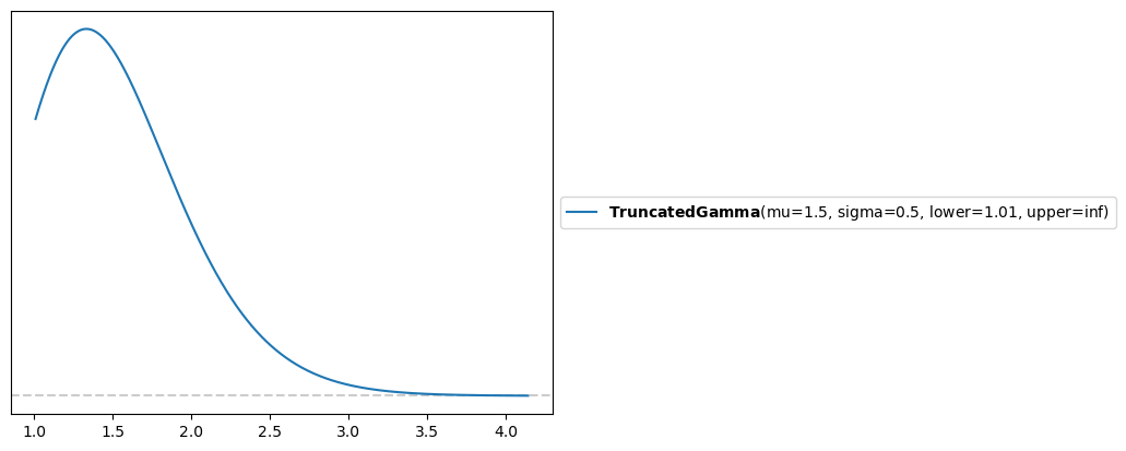
Alternatively, we can use the Truncated wrapper to truncate the support of an arbitrary distribution. Perhaps we want a Gamma distribution on \(\sigma_C\) (the Arrow-Pratt risk aversion), but we don’t want it to go below 1.01 (we’re ruling out the log case for numerical stability reasons). This can be accomplished as follows:
sigma_C ~ Truncated(Gamma(mu=1.5, sigma=0.5), lower=1.01, upper=None) = 1.5;
The prior implied by this configuration is plotted below:
pz.Truncated(pz.Gamma(mu=1.5, sigma=0.5), lower=1.01, upper=None).plot_pdf()
<Axes: >
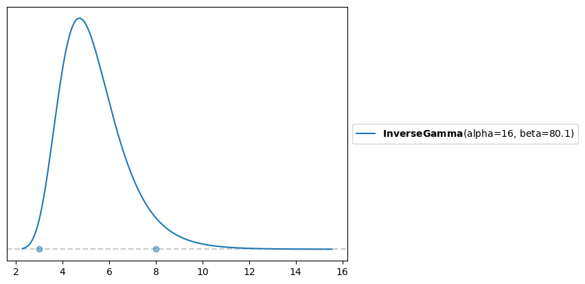
When working with many distributions, it is difficult to map you beliefs about plausable parameter values to hyperparameters for the prior. For example, suppose I do some research and find that values for the Arrow-Pratt risk aversion range between 3 and 8. What prior should be used?
In this case, pz.maxent can help. This function finds a distribution from a requested family such that 95% of the probability mass lies between two points. For example, we can find the Inverse Gamma distribution with 95% of the mass between 3 and 8. This turns out to be InverseGamma(alpha=16, beta=80.1).
You can directly use maxent inside of your GCN files. For example:
sigma_C ~ maxent(InverseGamma(), lower=3, upper=8) = 3.5
This makes it easier to share your model with other researchers. If we had written alpha=16, beta=80.1, I would be extremely confused. But seeing maxent(... lower=3, upper=8), it is immediately obvious what your prior beliefs about this parameter are.
pz.maxent(pz.InverseGamma(), lower=3, upper=8)
(InverseGamma(alpha=16, beta=80.1), <Axes: >)
file_path = "../GCN Files/RBC.gcn"
model = ge.model_from_gcn(file_path, verbose=True)
Model Building Complete.
Found:
	9 equations
	9 variables
		The following variables were eliminated at user request:
			TC_t, U_t
		The following "variables" were defined as constants and have been substituted away:
			mc_t
	1 stochastic shock
		 0 / 1 has a defined prior.
	6 parameters
		 6 / 6 parameters has a defined prior.
	0 parameters to calibrate.
Model appears well defined and ready to proceed to solving.
Initial values are whatever is given after the =, as explained above.
model.parameters()
{'alpha': 0.35,
 'beta': 0.99,
 'delta': 0.02,
 'rho_A': 0.95,
 'sigma_C': 1.5,
 'sigma_L': 2.0}
Priors are stored in model.param_priors for parameters, and model.shock_priors for shocks. In this case, we didn’t give any shock priors, so that’s an empty dictionary.
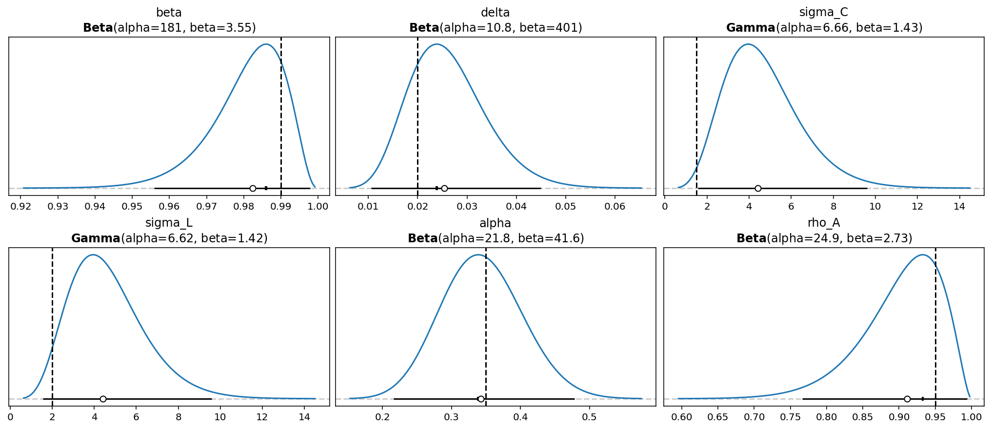
model.param_priors
{'beta': Beta(alpha=181, beta=3.55),
 'delta': Beta(alpha=10.8, beta=401),
 'sigma_C': Gamma(alpha=6.66, beta=1.43),
 'sigma_L': Gamma(alpha=6.62, beta=1.42),
 'alpha': Beta(alpha=21.8, beta=41.6),
 'rho_A': Beta(alpha=24.9, beta=2.73)}
model.shock_priors
{}
You can look at the priors set in the GCN file using gp.plot_priors. The inital value is marked with a veritcal line.
gp.plot_priors(model, n_cols=3, figsize=(14, 6));
ss_res = model.steady_state()
ge.print_steady_state(ss_res)
A_ss               1.000
C_ss               2.358
I_ss               0.715
K_ss              35.732
L_ss               0.820
Y_ss               3.073
lambda_ss          0.276
r_ss               0.030
w_ss               2.436
T, R = model.solve_model(steady_state=ss_res)
Solution found, sum of squared residuals: 0.000000000
Norm of deterministic part: 0.000000000
Norm of stochastic part: 0.000000000
Statespace Models#
Currently, support for using priors in a Model is limited. They are mostly used via the DSGEStateSpace class. This can be created using ge.statespace_from_gcn
ss_mod = ge.statespace_from_gcn(file_path)
Model Building Complete.
Found:
	9 equations
	9 variables
		The following variables were eliminated at user request:
			TC_t, U_t
		The following "variables" were defined as constants and have been substituted away:
			mc_t
	1 stochastic shock
		 0 / 1 has a defined prior.
	6 parameters
		 6 / 6 parameters has a defined prior.
	0 parameters to calibrate.
Model appears well defined and ready to proceed to solving.
Statespace model construction complete, but call the .configure method to finalize.
type(ss_mod)
gEconpy.model.statespace.DSGEStateSpace
A DSGEStateSpace is a bridge between your symbolic DSGE model and a PyMC model. To use it, first call the .configure method to set up some options. For more details on all the different options, see the introduction to estimation notebook
ss_mod.configure(
    observed_states=["Y"],
    measurement_error=None,
    solver="scan_cycle_reduction",
    max_iter=20,
    mode="JAX",
)
                  Model Requirements

  Variable          Shape   Constraints   Dimensions
 ────────────────────────────────────────────────────
  alpha             ()                          None
  beta              ()                          None
  delta             ()                          None
  rho_A             ()                          None
  sigma_C           ()      Positive            None
  sigma_L           ()      Positive            None
  sigma_epsilon_A   ()      Positive            None

 These parameters should be assigned priors inside a
         PyMC model block before calling the
            build_statespace_graph method.
Priors can then be loaded into a PyMC model using ss_mod.to_pymc(). Since we didn’t specify a prior for sigma_epsilon_A, we need to do that ourselves.
import pymc as pm

with pm.Model(coords=ss_mod.coords) as pm_model:
    ss_mod.to_pymc()
    sigma_epsilon_A = pm.Gamma("sigma_epsilon_A", alpha=2, beta=10)
To generate data, use ge.data_from_prior
true_params, data, prior = ge.data_from_prior(statepace_mod=ss_mod, pymc_model=pm_model, random_seed=rng)
/Users/jessegrabowski/mambaforge/envs/geconpy-dev/lib/python3.12/site-packages/pymc_extras/statespace/utils/data_tools.py:159: ImputationWarning: Provided data contains missing values and will be automatically imputed as hidden states during Kalman filtering.
  warnings.warn(impute_message, ImputationWarning)
Sampling: [alpha, beta, delta, obs, rho_A, sigma_C, sigma_L, sigma_epsilon_A]
Sampling: [prior_combined]
For each simulation, the prior.prior group saves the steady state error in a variable called ss_resid. Using that, we can check if any parameters cause us problems.
The maximum of this parameter is 1e-29, so all prior draws resulted in a valid steady-state solution.
prior.prior.ss_resid.max().item()
2.7353044381158726e-29
We can also check the solver errors. These are stored in two parts, stochastic_norm and deterministic_norm. Both sould be close to zero for valid model solutions. In this case, they each have a maximum of 1e-15, so no prior draws were associated with failures in computing the policy function.
prior.prior.stochastic_norm.max().item(), prior.prior.deterministic_norm.max().item()
(1.790194494725003e-15, 3.7021103646840064e-15)
One final diagnostic is the number of steps required for the cyclic reduciton algorithm to converge. This algorithm is used to compute the QZ decomposition used in solving the policy function. When it needs a lot of steps, it might indicate potentially unstable parameters.
In the .configure call, we set the maximum number of steps to 20. Among all prior draws, only a maximum of 12 was used.
prior.prior.n_cycle_steps.max().item()
12
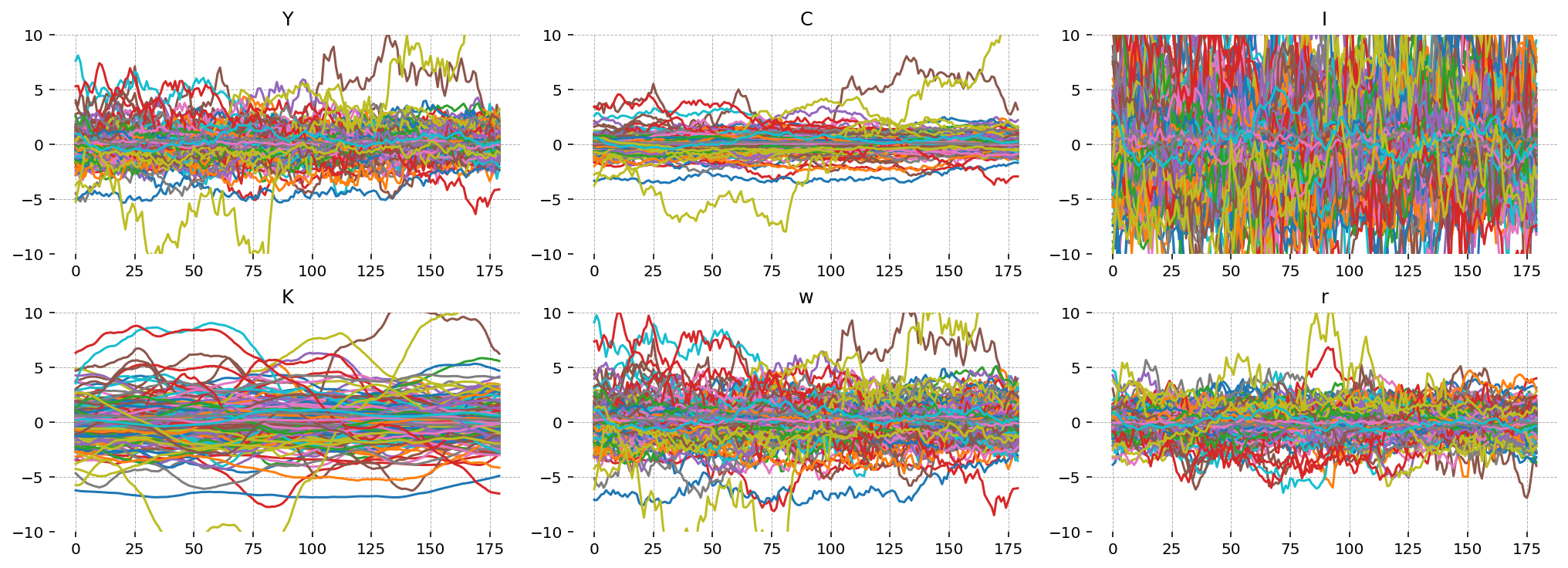
Plot Simulated Trajectories#
Finally, we can plot some simulated trajectories from the prior. This is equivalent to gp.plot_simulation, but now prior uncertainty about the true parameter values is being taken into account.
import matplotlib.pyplot as plt

gp.set_matplotlib_style()

fig = plt.figure(figsize=(14, 5), dpi=144)

gs, locs = gp.prepare_gridspec_figure(n_cols=3, n_plots=6, figure=fig)
for loc, var in zip(locs, ["Y", "C", "I", "K", "w", "r"], strict=False):
    axis = fig.add_subplot(gs[loc])
    axis.plot(
        np.arange(data.shape[0]),
        prior.unconditional_prior.prior_latent.sel(chain=0, state=var).values.T,
    )
    axis.set(title=var, ylim=(-10, 10))

plt.show()
Authors#
Authored by Jesse Grabowski in March 2025
Watermark#
%load_ext watermark
%watermark -n -u -v -iv -w -p gEconpy
Last updated: Sat Mar 15 2025

Python implementation: CPython
Python version       : 3.12.9
IPython version      : 9.0.1

gEconpy: 0+untagged.305.gd931e48.dirty

gEconpy   : 0+untagged.305.gd931e48.dirty
xarray    : 2025.1.2
numpy     : 1.26.4
pymc      : 5.21.1
pandas    : 2.2.3
preliz    : 0.15.0
matplotlib: 3.10.1

Watermark: 2.5.0