Time Aware Symbols#
The TimeAwareSymbol object is an extension of sympy.Symbol. It is an important building block of DSGE models. This short tutorial shows what they are, and how they can be used.
import sys

sys.path.append("/Users/jessegrabowski/Documents/Python/gEconpy/")
import sympy as sp

from gEconpy.classes.time_aware_symbol import TimeAwareSymbol
Basic Functionality#
A TimeAwareSymbol functions exactly like sp.Symbol, except that it accepts a time_index argument. time_index is an integer that gives an offset from time t. Here are three examples:
x_t = TimeAwareSymbol("x", time_index=0)
x_tm1 = TimeAwareSymbol("x", time_index=-1)
x_tp1 = TimeAwareSymbol("x", time_index=1)
x_t
x_tm1
x_tp1
The variable is build from the provided base_name (in this case x), and the time_index. The name is constructed by combining these two elements.
x_t.name
'x_t'
x_t.base_name
'x'
x_t.time_index
0
There is also a safe_name, which can be used in contexts where the + or - in the name would be problematic. For the safe_name, + is replaced with p, and - with m.
x_tp1.name
'x_t+1'
x_tp1.safe_name
'x_tp1'
x_tm1.safe_name
'x_tm1'
Otherwise, all other arguments to sp.Symbol can be specified. For example, assumptions are allowed:
x_t_positive = TimeAwareSymbol("x", time_index=0, positive=True)
x_t_positive
x_t_positive.assumptions0
{'positive': True,
 'finite': True,
 'negative': False,
 'commutative': True,
 'complex': True,
 'extended_positive': True,
 'imaginary': False,
 'extended_nonzero': True,
 'zero': False,
 'extended_nonpositive': False,
 'extended_real': True,
 'hermitian': True,
 'nonnegative': True,
 'nonzero': True,
 'nonpositive': False,
 'real': True,
 'extended_negative': False,
 'infinite': False,
 'extended_nonnegative': True}
Time manipulations#
After creation, several methods for manipulating the time index of the variable are available:
step_forwardincrements thetime_indexstep_backwarddecremetes thetime_indexset_tallowstime_indexto be set directly
x_t.step_forward()
x_t.step_backward()
The most important feature of TimeAwareSymbols is that when two TimeAwareSymbols have the same base_name and time_index, they evaulate as equal
x_t.step_backward() == x_tm1
True
x_t.step_forward() == x_tp1
True
Steady State#
Another important concept in analysis of dynamic systems is a “steady state”. A steady state is an equlibrium such that \(x_t = x_{t+1} = x_{t+1} = \dots = x_{ss}\)
Variables can be sent to the steady state using the to_ss method
x_t.to_ss()
Since ‘ss’ is a special time_index, variables of the same base_name sent to the steady state will evaluate to equal
x_t.to_ss() == x_tp1.to_ss()
True
Working with Equations#
TimeAwareSymbols subclass Symbol, so anything you can do with a symbol can be done with a TimeAwareSymbol.
For example, you can do algebraic manipulations
eq = sp.Eq(x_tp1, (x_t + x_tm1) / 2)
eq
Or call sympy.solve
sp.solve(eq, x_t)[0]
Usually, though, you are going to want to manipulate the time indices for entire expressions. Unfortunately, there is no TimeAwareExpr. Instead, gEconpy gives some helper functions for manipulation of equations that include TimeAwareSymbols. These are:
step_equation_forwardstep_equation_backwardeq_to_ss
The equations do what the names suggest
from gEconpy.utilities import (
    eq_to_ss,
    step_equation_backward,
    step_equation_forward,
)
step_equation_forward(eq)
step_equation_backward(eq)
eq_to_ss(eq.lhs - eq.rhs)
Example 1: \(AR(1)\) to \(MA(\infty)\)#
Using these tools, we can do powerful analysis on time series.
Consider an AR(1) system:
We can use step_equation_backward together with repeated substitution to derive the \(MA(\infty)\) form of the \(AR(1)\) system
eps_t = TimeAwareSymbol("\\varepsilon", 0)
rho = sp.Symbol("rho", positive=True)

# This is only the right-hand side, remember there's an x_t on the left
ar_1_rhs = rho * x_tm1 + eps_t
We will iterative shift the equation backwards and substitute
curr_x = x_t
curr_rhs = ar_1_rhs.copy()
for _ in range(10):
    display(sp.Eq(x_t, ar_1_rhs))
    curr_x = curr_x.step_backward()
    curr_rhs = step_equation_backward(curr_rhs)
    ar_1_rhs = ar_1_rhs.subs({curr_x: curr_rhs}).expand()
Since \(\rho \in (0, 1)\), the leading term will eventually go to zero, and we recover the well-known equation:
I don’t know any way for sympy to automatically detect the presence of this series and rewrite into summation notation – if you do, open an issue so I can update this example!
Example 2: Analytical Steady State#
More useful, perhaps, is that we can use TimeAwareSymbols to derive the steady state of a dynamical system. Consider the AR(1) equation again:
ar_1 = sp.Eq(x_t, rho * x_tm1 + eps_t)
ar_1
We can send this to the steady-state and compute the value of \(x_{ss}\)
sp.solve(eq_to_ss(ar_1), x_t.to_ss())[0]
Obviously we need to know something about \(\varepsilon_{ss}\). We typtically assume \(\varepsilon_t ~ N(0, \sigma)\). In the (deterministic!) steady state, there are no shocks, so \(\varepsilon_{ss} = 0\).
Let’s generalize the equation to allow a drift in the shocks, so \(\varepsilon_t ~ N(\mu, \sigma)\). We can pull out the \(\mu\) using the properties of normal distributions to obtain:
mu = sp.Symbol("mu")
ar_1 = sp.Eq(x_t, mu + rho * x_tm1 + eps_t)
ar_1
Solving for the steady state gives the well-known expression for the AR(1) steady state
sp.solve(eq_to_ss(ar_1).subs({eps_t.to_ss(): 0}), x_t.to_ss())[0]
Example 3: Deterministic RBC#
Consider an RBC model defined (in reduced form) as follows:
C, K, A, epsilon = [TimeAwareSymbol(x, 0) for x in ["C", "K", "A", "\\varepsilon"]]
alpha, beta, delta, rho = sp.symbols(
    "alpha beta delta rho",
)

euler = C.step_forward() / C - beta * (alpha * sp.exp(A.step_forward()) * K.step_forward() ** (alpha - 1) + 1 - delta)
transition = K.step_forward() - (sp.exp(A) * K**alpha + (1 - delta) * K - C)
shock = A - rho * A.step_backward() - epsilon

system = [euler, transition, shock]
for eq in system:
    display(eq)
We can use TimeAwareSymbols to solve for the deterministic steady state of this entire system in one fell swoop
ss_system = [eq_to_ss(eq).simplify().subs({epsilon.to_ss(): 0.0}) for eq in system]
ss_dict = sp.solve(ss_system, [K.to_ss(), C.to_ss(), A.to_ss()], dict=True)[0]

for var, eq in ss_dict.items():
    display(sp.Eq(var, eq))
Using sp.lambdify, we can compile a function that computes the steady state of the system given input parameters. This is essentially what gEconpy does internally when solving for the steady state of a DSGE model.
f_ss = sp.lambdify([alpha, beta, delta, rho], list(ss_dict.values()))
param_dict = {"alpha": 0.33, "beta": 0.99, "delta": 0.035, "rho": 0.95}
f_ss(**param_dict)
[0, 1.9825902234443513, 19.50030034168597]
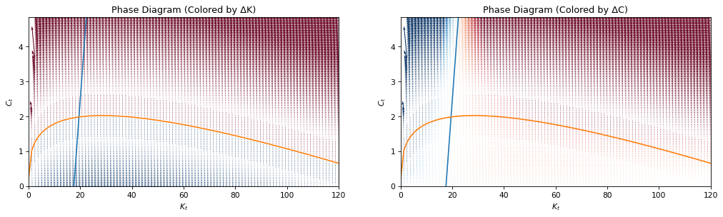
Phase Diagram#
Since this system is deterministic, we can construct a phase diagram showing system dynamics for a given \((C_t, K_t)\) tuple. To do this, we first need to re-arrange the Euler equation and law of motion of capital to obtain rates of change, \(\Delta C_{t+1}\) and \(\Delta K_{t+1}\). For \(\Delta C_{t+1}\) we get:
For the second line, the Euler equation was solved for \(C_{t+1}\) and substituted.
For \(\Delta K_{t+1}\):
Computing these \(\Delta\)s over a grid of points will give us a phase diagram. Let’s look at how these can be solved for with sympy:
C_tp1 = sp.solve(euler, C.set_t(1))[0]
C_tp1
Delta_C = (C_tp1 - C).collect(C).subs({A.set_t(1): 0})
Delta_C
This solution isn’t exactly what we need, though, because we don’t want the \(K_{t+1}\). Use the transition equation to write it in terms of time \(t\) variables only
K_tp1 = sp.solve(transition.subs({A: 0}), K.set_t(1))[0]
Delta_C = Delta_C.subs({K.set_t(1): K_tp1})
Delta_C
K_tp1 = sp.solve(transition, K.set_t(1))[0].subs({A: 0})
K_tp1
Delta_K = K_tp1 - K
Delta_K
Compile a function with sp.lambdify
parameters = list(param_dict.keys())
f_Delta = sp.lambdify([C, K, *parameters], [Delta_C, Delta_K])
We are also interested in when \(\Delta C_{t+1} = \Delta K_{t+1} = 0\), because these equations will form boundaries in phase space. We can do this by using sp.solve.
First, solve \(\Delta C_{t+1}\) for \(C_t\). There will be two solutions, and one will be zero (since the whole expression is multiplied by \(C_t\)). We’re only interested in the non-trivial solution.
boundary_1 = sp.solve(Delta_C, C)[1]
boundary_1
Next, solve \(\Delta K_{t+1}\) for \(C_t\)
boundary_2 = sp.solve(Delta_K, C)[0]
boundary_2
Compile a function
f_boundaries = sp.lambdify([K, *parameters], [boundary_1, boundary_2])
Functions created with sp.lambdify are inherently vectorized, so we can make a grid of capital values and compute the associated consumpions
import matplotlib.pyplot as plt
import numpy as np

k_max = 120
c_max = k_max ** param_dict["alpha"]  # We can't consume more than exists in the economy!

k_grid = np.linspace(1e-2, k_max, 100)
c_grid = np.linspace(1e-2, c_max, 100)
boundaries = f_boundaries(k_grid, **param_dict)

kk, cc = np.meshgrid(k_grid, c_grid)
with np.errstate(divide="ignore", invalid="ignore"):
    c_delta, k_delta = f_Delta(cc, kk, **param_dict)
fig, ax = plt.subplots(1, 2, figsize=(16, 4), dpi=77)
for axis, colorby, name in zip(fig.axes, [k_delta, c_delta], ["ΔK", "ΔC"], strict=False):
    axis.plot(k_grid, boundaries[0], label="ΔK = 0")
    axis.plot(k_grid, boundaries[1], label="ΔC = 0")
    quiver_plot = axis.quiver(kk, cc, k_delta, c_delta, colorby, cmap=plt.cm.RdBu, clim=(-0.05, 0.05))
    axis.set(
        xlim=(0, k_max),
        ylim=(0, c_max),
        xlabel="$K_t$",
        ylabel="$C_t$",
        title=f"Phase Diagram (Colored by {name})",
    )
plt.show()
Authors#
Authored by Jesse Grabowski in March 2025
Watermark#
%load_ext watermark
# Delete lambdify functions (they break watermark)
del f_ss, f_Delta, f_boundaries

%watermark -n -u -v -iv -w -p gEconpy
Last updated: Sat Mar 15 2025

Python implementation: CPython
Python version       : 3.12.9
IPython version      : 9.0.1

gEconpy: 0+untagged.305.gd931e48.dirty

sympy     : 1.12.1
sys       : 3.12.9 | packaged by conda-forge | (main, Feb 14 2025, 07:56:32) [Clang 18.1.8 ]
gEconpy   : 0+untagged.305.gd931e48.dirty
numpy     : 1.26.4
matplotlib: 3.10.1

Watermark: 2.5.0